Areal Surface Texture Analysis

Areal Surface Texture Analysis for Both the Lab and the Engineer's Desk

March 7, 2019

Over the last two decades a number of software packages have been developed for analyzing areal surface texture and its impact on component functionality. These software packages have, however, almost exclusively been geared toward metrology professionals with an intimate knowledge of surface texture analysis. The packages present users with a vast number of tools, which can be intimidating and difficult to grasp without significant guidance. Furthermore, it isn’t always clear how applying the tools and changing parameters is actually affecting the datasets.

All too often, the people who understand the analysis software are far removed from those that are connected with designing and specifying the surfaces Thus, the design, manufacturing and quality engineers, who could also benefit from these tools, must rely on their lab to interpret surface texture data for them, rather than being able to interact with the data itself. The result is that engineers continue to specify only the most basic, but well understood, surface parameters, such as average roughness, whether those parameters are useful or not.

A new software approach for surface texture analysis is now available, providing an analysis experience that can be shared by both engineers and lab professionals to truly understand, communicate and improve surface functionality. By introducing a step-by-step and visual approach to texture analysis, the software allows designers, managers and process engineers to explore surface texture and communicate both graphically and numerically.

In this paper we present this step-by-step process of analyzing surface data. We will show how Digital Metrology’s OmniSurf3D software visually presents each of the steps in a language both engineers and quality professionals can use to understand and improve component performance.

OmniSurf3D software provides visual and numerical representations of 3D surface texture — *OmniSurf3D software. The 3D surface is shown in color. The large-scale tilt of the surface is shown as a transparent, blue plane.*

Surface Analysis Augments Instinctive Understanding

The most powerful surface analysis tools are the human eye and the human brain. Thousands of times per day we look at surfaces and intuitively determine if they are rough, smooth, safe to walk on, dangerous to touch, nice to look at, etc.

Areal (or “3D”) surface texture measurements with proper data visualization tools can provide a link between a technical measurement and the power of human interpretation. Unfortunately, in most companies there is a problem: those responsible for designing, developing and manufacturing surfaces are not necessarily those that actually explore the measurement data. In many cases, those that work outside the laboratories simply get a number such as “form error” or “RMS roughness” from a lab and this limited information is all that they have for driving their designs and decision making.

With today’s tools it is possible for the laboratory to measure and store topography data which designers and engineers can subsequently explore and analyze at their desks. This is an optimal approach. It allows the quality laboratory to focus on its expertise of providing accurate data while the engineering department can leverage its product knowledge.

The challenge of moving surface analysis tools out of the lab and into the engineers’ offices is that the software tools must be intuitive and descriptive. Today’s engineers are required to be experts in many disciplines; surface analysis must therefore be an informative tool for exploration rather than an additional burden.

The Basic Steps for Analyzing Surface Textures

The process of exploring and analyzing areal surface texture can be considered as four fundamental activities:

1. Cleaning up, or pre-processing, the data
2. Accounting for the nominal geometry
3. Extracting the surface features or shapes of interest via filtering
4. Describing the features of interest with numerical parameters.

These four steps will be addressed in more detail in the following sections. Well-constructed analysis software makes it possible to explore any or all of these areas while not requiring the user to adhere to a lengthy, rigid process in order to obtain meaningful results.

1. Cleaning Up (Pre-Processing) the Dataset

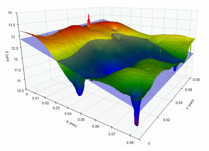
Surface data may be acquired by many different instruments, ranging for mechanical stylus profilers through optical, 3D (areal) measurement systems. With a 2D stylus-based system, the sensor always knows the stylus position as it moves up and down along a surface. However, in optical measurement, this isn’t always the case. Sometimes an optical measurement system will not detect data at certain pixels–perhaps due to steep slopes or surface contamination. In other cases, the optical instrument may misrepresent the height of individual pixels due to other imaging or detection problems, resulting in outliers. Some examples are shown here:

3D surface texture measurement with missing points due to steep slopes. — *Missing points due to steep slopes.*

surface texture measurement with outliers due to sensor not properly detecting pixels. — *Outliers due to sensor not properly detecting pixels.*

The first step in the analysis process, then, is to account for errors in the data such as missing points and outlying data. OmniSurf3D provides tools to easily account for errors in the incoming data without inadvertently altering the data itself and thus skewing the surface parameters.

Addressing Missing Points

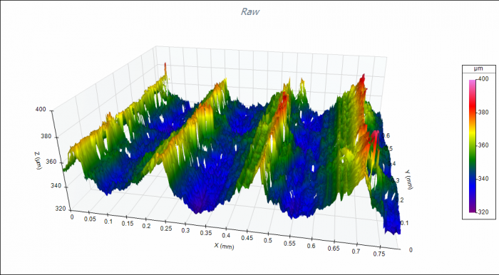
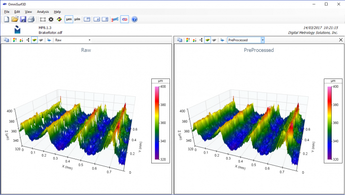
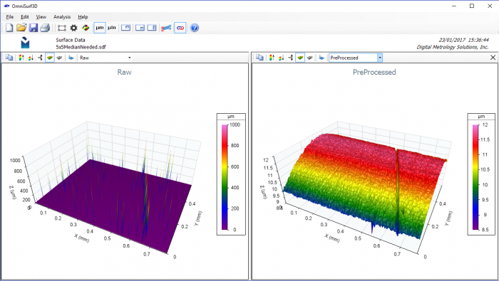
Missing points can be filled by various interpolation methods. Interpolation can provide better visualizations and, when done correctly, will have minimal impact on computed parameters. In the example shown below, the very fast, bi-linear interpolation method is used to predict the height of missing points based on their neighboring valid heights.

OmniSurf3D provides “dual visualization” views for fast comparison as analysis features are applied. Here, the raw data is shown on the left of the dual view, while the data on the right has been pre-processed with the missing points filled with interpolated values.

Bi-linear filling of missing data. OmniSurf3D’s dual visualization shows the pre-processed data on the left and the processed data on the right, clearly showing the effect of the operation. Image Courtesy Michigan Metrology.

Addressing Outlying Points

Outlying points can be dealt with by various approaches depending on the types of outliers. The most common method for correcting “single pixel” outliers is the median filter. The median filter looks at a square of pixels (typically 3×3 or 5×5) centered at the pixel of interest. The center pixel is replaced by the median of the pixels (typically 9 or 25) contained in the square.

For example, an outlying point with the height of “10” has these 3×3 neighbors:

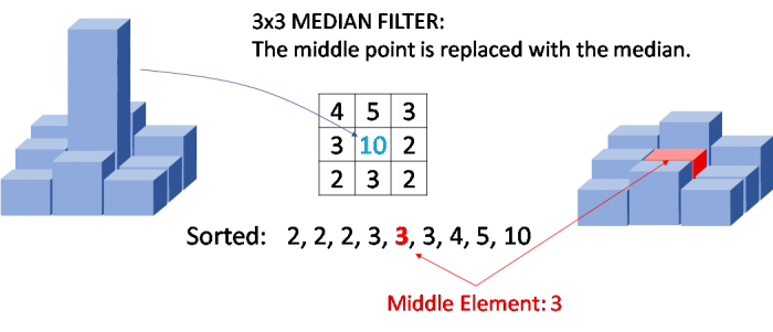
3x3 Median filtering. The center pixel of a 3x3 square is replaced with the median of its neighbors to remove single-pixel outliers. — *3×3 Median filtering. The center pixel of a 3×3 square is replaced with the median of its neighbors to remove single-pixel outliers.*

The 3×3 median filter sorts all nine of the heights and replaces the middle pixel’s height (previously “10”) with the median value “3”. The median filter’s “square” is passed over the entire image resulting in the removal of “single pixel noise”. Once again, we can see the effects of this filter via the OmniSurf3D dual visualization view shown below. Note that when the outlying data points (left) are removed, the true structure of the surface becomes apparent (right).

Median filtering to remove outlying points. OmniSurf3D’s dual visualization shows how the outlying data suppresses the actual shape of the surface. Once these outliers are removed, the overall cylinder becomes apparent. — Median filtering to remove outlying points. OmniSurf3D’s dual visualization shows (on the left) how the outlying data suppresses the actual shape of the surface. Once these outliers are removed, the overall cylinder (right) becomes apparent.

Other methods are available to address outliers in measured data sets. In some cases, simple threshold based methods (with deletion of adjacent regions) can be useful. In other cases “Robust” filtering, can be a powerful tool for outlier suppression.

2. Accounting for the Nominal Geometry

To properly explore the height and depth of the “texture” of a surface we need to be able to separate the texture features from the underlying geometry. For example, it is difficult to visualize and describe the coating nodules on this spherical surface (left image) until the underlying spherical shape has been removed (as shown in the right image).

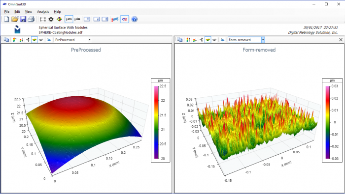
The nodules on this spherical surface are difficult to discern relative to the underlying shape of the surface. By removing the spherical shape, the fine features can be visualized and quantified . — The nodules on this spherical surface are difficult to discern relative to the underlying shape of the surface (left). By removing the spherical shape, the fine features can be visualized and quantified (right). Note the scaling differences between the two images.

Geometry removal is considered as the “F” or “form removal” operation in the ISO 25178 series of standards which govern how surface data should be collected and reported. For the analysis of measured data sets, it makes the most sense to first remove the underlying geometry in order to better visualize the influence of the filtering operations.

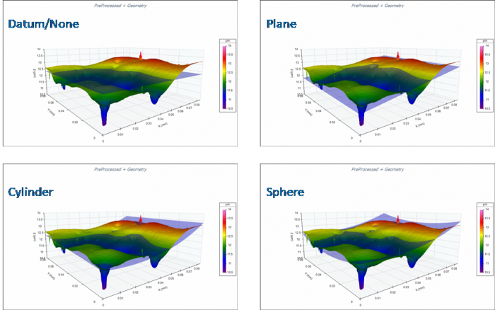
In OmniSurf3D, several reference geometries (forms) can be removed from the surface data. These include planes, cylinders, cones, spheres, aspherics, polynomial surfaces, etc. The selection is based on knowledge of the underlying geometry. For example, if the surface is designed to be flat/planar, then a plane should be used as the reference geometry. If the surface is designed to be cylindrical, a cylinder should be used. In some cases the surface shape is not of a primitive geometry; in many of these cases, polynomials can be very useful for approximating the underlying shape.

The ability to visualize how a reference geometry relates to the measured surface is important for properly extracting and understanding surface features. For example, it would seem natural to treat a sample of fabric or paper as essentially planar; however, if the sample is bunched or curved, then applying a reference plane may distort the data, where a polynomial surface fit would not. OmniSurf3D can display the reference geometry as a transparent surface cutting through the part surface, making it easy to see how appropriately the reference matches the actual data. Some examples are shown below:

*OmniSurf3D’s visualization of reference geometry fitting. The ability to see how well the reference geometry fits the actual data helps a user to choose the most appropriate shape removal.*

3. Extracting the Surface Features or Shapes of Interest Via Filtering

Surfaces are made up of features occurring at varying scales, or wavelengths. For example, a road surface is made up of many different wavelengths:

surface texture wavelength regimes can be compared to the surface roughness and waviness of a road surface. — *The many wavelength regimes of a road, ranging from the texture on the sides of the gravel (short wavelengths) to large hills and valleys (long wavelengths).*

To explore a specific wavelength region of interest we must apply filtering to limit or “bound” the wavelength band of interest. In the context of ISO 25178 the application of a short wavelength limiting filter is referred to as the “S” operation. The application of a long wavelength limiting filter is referred to as the “L” operation. These filters (operators) can be adjusted to extract various shapes from a surface. For example, many surface texture reference books speak of the surface domains: roughness, waviness and form.

*The common 3-domain approach to surface texture: roughness, waviness and form.*

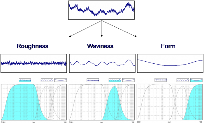
Under this 3-domain approach the measured surface is separated into three surfaces–each of which could be related to various functional or process-related implications. In the above figure we have a milled surface analyzed as follows:

• Roughness: S-L (short–long) limited surface

• Waviness: S-L (short–long) limited surface

• Form: S-F (short–form) limited surface

To define a filter, we must specify two things: a cutoff wavelength and a filter type.

The cutoff wavelength defines the point where the data is separated into long (waviness) and short (roughness) wavelengths. The cutoff wavelength can be described as “the amount of smoothing” that goes into the waviness side of the filter. We can see the influence of the filter cutoff wavelength selection in the following figure:

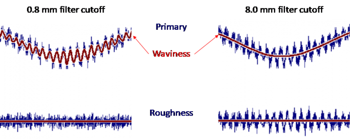
The impact of the cutoff wavelength selection. Note that the 0.8 mm cutoff (left) results in a waviness profile with many peaks and valleys. The 8.0 mm cutoff (right) smooths the waviness profile into a single curve while also introducing larger wavelength structure in the roughness profile.

In the above example, we have a primary surface profile (the blue data on top) shown twice. On the left, the primary profile is filtered with a relatively small cutoff value (0.8 mm). This gives a waviness profile (top left red profile) with several peaks and valleys. The roughness profile on the bottom left is what remains if we remove the left waviness profile from the primary profile.

Similarly, on the top right we have a waviness profile based on a larger (8.0 mm) filter cutoff value. This larger cutoff value creates a smoother waviness profile and as a result, there is an increase in roughness in the lower right graph.

The other aspect of the filter that must be selected is the filter type. This defines the way that the smoothing occurs. Typical filter types are Gaussian and Robust. The Gaussian filter is the most common filter and suits the widest variety of applications. It is based on a Gaussian (or “bell curve”) shaped moving average that runs through the data to create a waviness profile or surface:

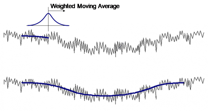
surface texture - a Gaussian filter provides a weighted moving average. — *The Gaussian filter.*

Robust filtering should be considered when outlying features cause unwanted distortions in the data. These distortions with the Gaussian filter can occur with surfaces containing porosity or scratches.

Choosing the filter’s cutoff wavelength (also called the filter’s “nesting index” in the ISO 25178 series) is essential in extracting the features of interest. OmniSurf3D provides a variety of visualization tools to help the user understand the filter’s influence and better understand the surface being studied.

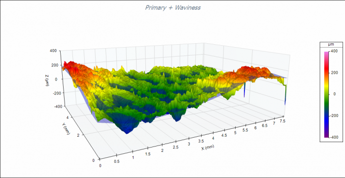
The Short Filter (S operator)

The short filter suppresses (removes) the unwanted short wavelengths from the Geometry Suppressed surface. The resulting surface is called the “Primary” surface. The amount of filtering is set by the short filter’s cutoff wavelength (nesting index).

This example shows a form suppressed surface and associated Primary surface based on a 0.080 mm short filter.

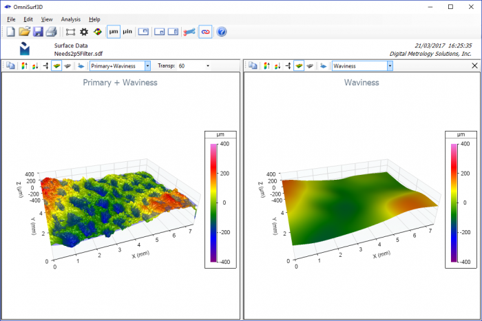
The application of the short filter. Note the loss of fine details in the Primary surface—at this wavelength scale, the filter has removed noise from the data to reveal the roughness. — *The application of the short filter. Note the loss of fine details in the Primary surface—at this wavelength scale, the filter has removed noise from the data to reveal the roughness (right).*

The Long Filter (L operator)

The long filter (L operator) establishes the surface wavelengths that go into the Waviness surface. This Waviness surface is removed in order to obtain the filtered (roughness) surface. The selection of this filter type and cutoff wavelength (nesting index) is very important as it can have a significant impact on computed parameters.

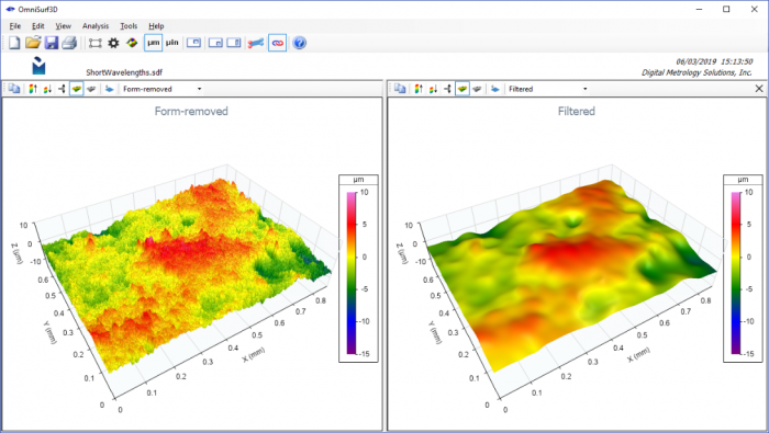
Given the importance of this filter selection, OmniSurf3D provides several visualization tools to aid the user in understanding and exploring the impact of the filter:

• A transparent Waviness surface plot. This visualization allows the user to see how the Waviness surface “fits” into the Primary surface.

surface texture - waviness surface shown inside the solid primary surface. — *A transparent Waviness surface shown inside the solid Primary surface.*

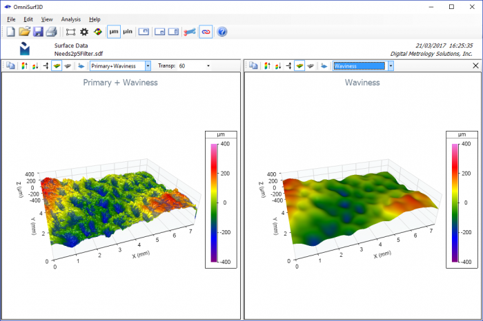
• Dual Visualization of Surface Plots

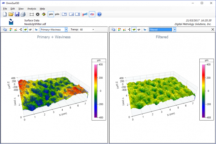
surface texture - OmniSurf3D’s dual visualization of the Primary-Waviness and Waviness surfaces. — *OmniSurf3D’s dual visualization of the Primary/Waviness (left) and Waviness (right) surfaces.*

surface texture - OmniSurf3D’s dual visualization of the primary-waviness surface and filtered roughness surface. — *OmniSurf3D’s dual visualization of the Primary/Waviness surface (left) and filtered Roughness surface (right).*

This visualization allows the user to quickly see how the filter is working on your data. For example, if the cutoff wavelength is set to a smaller value, we can easily see that the surface’s pockets begin to appear in the waviness domain. This means that the reported surface texture parameters will be missing these pockets:

surface texture - OmniSurf3D’s dual visualization of the primary surface and waviness surface. The presence of the finer “pockets” in the waviness may indicate a cutoff value that is too short. — *OmniSurf3D’s dual visualization of the Primary surface (left) and Waviness surface (right). The presence of the finer “pockets” in the waviness may indicate a cutoff value that is too short.*

4. Numerically Describing the Features of Interest

Beyond the visualization and exploration of surface data, we do ultimately need numbers in order to describe and control our surfaces. Without numerical values, we would have a difficult time establishing tolerances and controlling manufacturing processes. We would have no way of assessing quality. However, we should keep in mind:

Using a number to describe a surface’s shape
is like using decibels to describe a symphony:
there is much more information than can be contained in a single number.

Thus, we should first start with a visual and functional understanding of the surface. This understanding should drive the selection of numerical values. There are many different parameters that can be calculated for a surface–far more than can be described here. The best reference is ISO 25178-2. For this introduction, a few basic analysis categories and parameters will be presented.

Note: The most common height or “roughness” parameter for 2D profile analysis is the “Ra” (average roughness) parameter. In areal/3D surface texture, we do not have the “R” (roughness) or “W” (waviness) designations as we do not have the concept of roughness or waviness. In areal/3D surface texture we simply use the letter “S” to designate a surface. The “S” surface is made up of a controlled set of surface wavelengths that are determined by the S (short filter) and/or L (long filter) and/or F (form) operators.

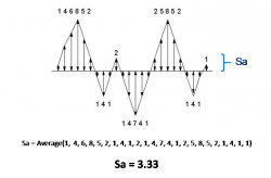
Describing Surface Heights
The most common areal parameter is the Sa (average roughness) value which is similar to the profile-based “Ra” value. This value is the average distance from the mean line based on all the data points.

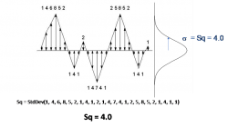
surface texture - the average roughness Sa value is based on average distances to the mean line. — *The Sa value based on average distances to the mean line.*

Another height description that is gaining popularity in 3D surface analysis is the Sq parameter. Mathematically this is the standard deviation of the surface heights and is therefore more useful in mathematical/statistical modelling.

surface texture - the root mean square RMS average roughness Sq value is based on the standard deviation of heights. — *The Sq value based on the standard deviation of heights.*

Describing the Surface Interface Area

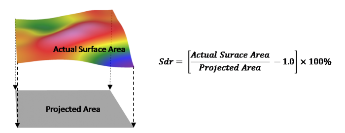
Whereas Sa and Sq describe heights, other parameters describe different, perhaps important aspects of the surface. For example, “Sdr”—the Developed Interface Ratio—describes the amount of surface area due to roughness as compared to the area if there were no roughness. The reported values is the percent of area gained due to the roughness.

surface texture - the Developed Interface Ratio Sdr value reporting the increase in surface area due to roughness. — *The Sdr value reporting the increase in surface area due to roughness.*

Describing Local Features

Areal “feature” extraction methods can detect and isolate features like peaks, pits, saddles, ridge lines and course lines:

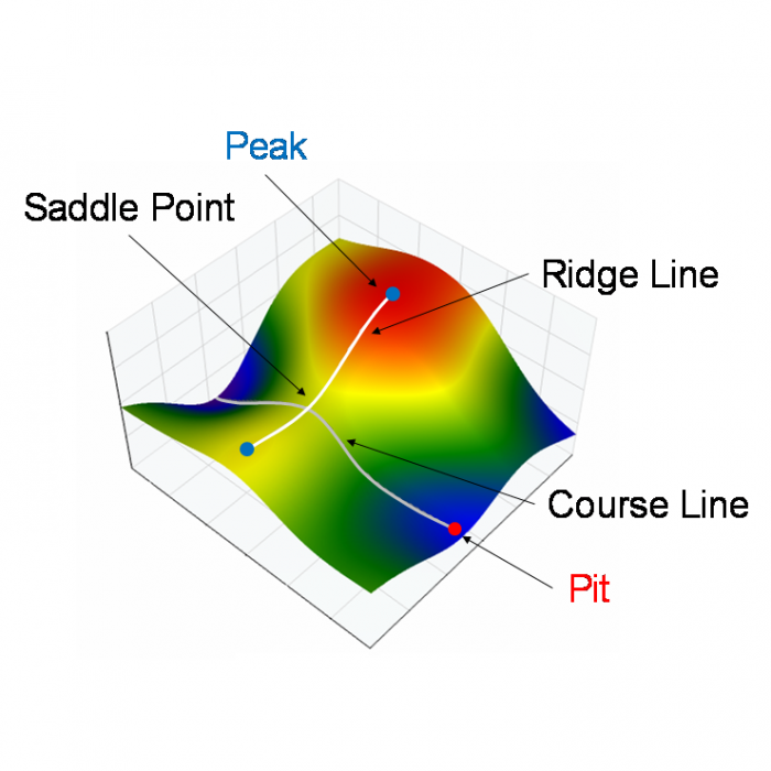
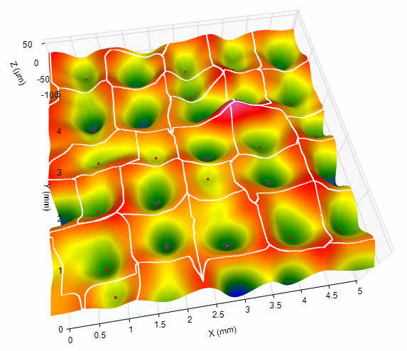
surface texture - OmniSurf3D software shows the peaks, ridge lines, saddle points, course lines and pits in a surface. — *Local features in areal topography.*

The area around a peak is classified as a “hill” and the area around a pit is classified as a “dale”. Statistics can be derived from these features such as average dale volume or average peak density. These parameters can be useful to describe how well a surface may hold lubricant or ink, or how the surface may slide or stick. Along with many parameters based on the detected features, OmniSurf3D provides a unique 3D visualization of these features for measured surfaces:

surface texture - OmniSurf3D software displays ridge lines and local pits. — *OmniSurf3D’s display of ridge lines and local pits.*

Additional Analysis Tools

In addition to the general surface parameters described above, lab professionals may access a broad body of tools to further analyze surfaces and correlate their texture to functionality.
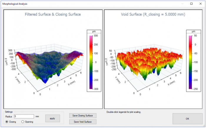
Morphological Analysis predicts how a soft surface will conform to a rigid surface. It is also useful as a tool to highlight sharp upward or downward features in a measured surface.

A morphological “closing” filter can be applied to a dataset to simulate a soft surface (e.g., a gasket) being pressed into a surface. This analysis method allows an engineer to explore surface functionalities such as the leakage under a gasket or the presence of stress-causing valleys or cracks.

Conversely, a morphological “opening filter” can be applied to show how peaks on the surface may relate to contact stresses, oil film penetration and cosmetic defects.
OmniSurf3D provides an interactive, extremely fast tool for applying morphological filtering and visualizing the gaps/voids or peaks.

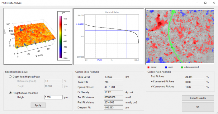
surface texture - OmniSurf3D software morphological analysis. A closing operation highlights the gaps and voids in the surface. — *OmniSurf3D’s morphological analysis. Here, a closing operation highlights the gaps/voids in the surface.*

Pit/Porosity analysis provides a wealth of information regarding pores and voids in a surface. OmniSurf3D provide tools for interactively slicing a surface to view and generate statistics on the detected pores. Furthermore, the “connectivity analysis” (shown in green in the image below) highlights features that may be potential leak paths:

surface texture - OmniSurf3D software Pit and Pore analysis. — *OmniSurf3D’s Pit/Pore analysis.*

Conclusion
The ability to measure, analyze and interpret surface texture data has opened vast possibilities for designing highly functional surfaces and controlling the processes required to manufacture them. By providing intuitive, efficient and informative tools for exploring surface texture, OmniSurf3D provides a common platform for surface analysis across all engineering functions. Designers can explore surface data directly to improve surface function early in the process, while quality and process engineers can dig deeper to discover the root causes of variation and to better control manufacturing for repeatable, reliable component function.